Predictive analytics

Predictive analytics

• 2.
  Evolution of Predictive Analytics
• 3.
  What is PredictiveAnalytics? Predictive analytics is the practice of extracting insights from the existing data set with the help data mining, statistical modeling and machine learning techniques and using it to predict unobserved/unknown events.  Identifying cause-effect relationships across the variables from the historical data.  Discovering hidden insights and patterns with the help of data mining techniques.  Apply observed patterns to unknowns in the Past, Present or Future.
• 4.
  What is PredictiveAnalytics
• 5.
  Predictive Analytics ProcessCycle
• 6.
  Analytics & PredictiveAnalytics  Analytics is the understanding of existing (retrospective) data with the goal of understanding trends via comparison  Developing analytics is the first step towards deriving predictive analytics  Predictive Analytics are more sophisticated analytics that “forward thinking” in nature  used for gaining insights from mathematical and/or financial modeling by enhancing understanding, interpretation and judgment for the purpose of good decision making
• 7.
  © 2011 PredictiveDashboards LLC 7 Comparative Study:: Analytics and Predictive Analytics Attribute Analytics Predictive Analytics Purpose: Understand the Past Observe Trends Catalyst for Discussion Gain Insights Make Decisions Take Action View: Historical and Current Future Oriented Metrics Type: Lagging Indicators Leading Indicators Data Used: Raw & Compiled Information Data Type: Structured Structured and Unstructured Users: Middle & Senior Mgt Analysts, End Users C-Level & Senior Mgt Strategists, Analysts, Mgrs Benefits: Gaining an understanding of data Productivity Improvements Gaining Information & Insights Process Improvements
• 8.
  Benefits Benefits of Analytics: productivitygains through improved data- gathering processes results in less time required for producing reports and metrics beneficial Not scalable, not repeatable Benefits of predictive analytics: process improvement gains through improve revenue generation & cost structures enhanced decision making Beneficial, Scalable, repeatable
• 9.
  Common Predictive Analytics •Regression:  Predicting output variable using its cause-effect relationship with input variables. OLS Regression, GLM, Random forests, ANN etc. • Classification: Predicting the item class. Decision Tree, Logistic Regression, ANN, SVM, Naïve Bayes classifier etc. • Time Series Forecasting: Predicting future time events given past history. AR, MA, ARIMA, Triple Exponential Smoothing, Holt- Winters etc. Contd.,
• 10.
  Common Predictive Analytics •Association rule mining: Mining items occurring together. Apriori Algorithm. • Clustering: Finding natural groups or clusters in the data. K- means, Hierarchical, Spectral, Density based EM algorithm Clustering etc. • Text mining: Model and structure the information content of textual sources. Sentiment Analysis, NLP
• 11.
  Regression  A RegressionModel defines three types of regression models:  linear,  Polynomial or Multiple regression  logistic regression. Or log linear regression
• 12.
  Linear Regression • Thesimplest form of regression to visualize is linear regression with a single predictor. A linear regression technique can be used if the relationship between x and y can be approximated with a straight line Y =  +  X
• 13.
  Nonlinear Regression • therelationship between x and y cannot be approximated with a straight line. In this case, a nonlinear regression technique may be used. Alternatively, the data could be preprocessed to make the relationship linear.
• 14.
  Multivariate Regression • Multivariateregression refers to regression with multiple predictors (x1 , x2 , ..., xn). For purposes of illustration Y = b0 + b1 X1 + b2 X2.
• 15.
  Decision Tree Induction •A decision tree is a structure that includes a root node, branches, and leaf nodes. • Each internal node denotes a test on an attribute, • Each branch denotes the outcome of a test, and • Each leaf node holds a class label. • The topmost node in the tree is the root node.
• 16.
  Balanced Decision Tree
• 17.
  Decision Tree Issues •Choosing Splitting Attributes • Ordering of Splitting Attributes • Splits (No. of Splits to take) • Tree Structure (few levels are required for a balanced tree) • Stopping Criteria – once training data is perfectly classified tree will stop – Stopping earlier results overfitting • Training Data – Neither too small nor too big • Pruning – improving of tree is needed by removing sub-trees when required
• 18.
  Entropy • Entorpy Itis the measure of disorder in a data set or amount of uncertainty in the dataset H(S) H (S) = • S – The current data set for which entropy is being calculated (change for every iteration of the ID3 algorithm • X – Set of classes in S • p(x) - It shows the ratio of number of elements in a class x with reference to number of elements of set S
• 19.
  Here our Partitionis on Colour not on Shapes . After partition we get
• 20.
  After partition 24 stars,25 Diamonds i.e., 24+25 = 49
• 21.
  Entropy • Entropy iscalculated for all stars and all diamonds
• 22.
  Entropy
• 23.
  Entropy
• 25.
  Information Gain • Informationgain is a measure of the decrease of disorder achieved by partitioning the original data set
• 26.
  CART • Create BinaryTree • Uses entropy • Formula to choose split point, s, for node t: • PL,PR probability that a tuple in the training set will be on the left or right side of the tree.
• 27.
  CART Example • Atthe start, there are six choices for split point (right branch on equality): – P(Gender)=2(6/15)(9/15)(2/15 + 4/15 + 3/15)=0.224 – P(1.6) = 0 – P(1.7) = 2(2/15)(13/15)(0 + 8/15 + 3/15) = 0.169 – P(1.8) = 2(5/15)(10/15)(4/15 + 6/15 + 3/15) = 0.385 – P(1.9) = 2(9/15)(6/15)(4/15 + 2/15 + 3/15) = 0.256 – P(2.0) = 2(12/15)(3/15)(4/15 + 8/15 + 3/15) = 0.32 • Split at 1.8
• 28.
  What is aNeural Network • A computer system modeled on the human brain and nervous system • NN is usually organized in layers • Layers are made up of number of inter- connected nodes • The connection strengths of neurons are called weights, that are used to store the acquired information (training examples)
• 29.
  Contd..Neural Networks • Duringthe learning process the weights are modified in order to model the particular learning task correctly on the training examples.
• 30.
  Propagation Tuple Input Output Input
• 31.
  CLASSIFICATION (RULE BASED)
• 32.
  Classification Using Rules •Perform classification using If-Then rules • Classification Rule: r = <a,c> Antecedent, Consequent • May generate from from other techniques (DT, NN) or generate directly. • Algorithms: Gen, RX, 1R, PRISM
• 33.
  Generating Rules Example
• 34.
  CLASSIFICATION TREES (ENSEMBLED METHODS)
• 35.
  Ensemble Methods • Ensemblemeans collection of large number of replicas (or mental copies or virtual copies), of the microstate of the system under macroscopic condition or • ensembling is a technique of combining two or more algorithms of similar or dissimilar types called base learners, • that incorporates predictions from base learners Contd.,
• 36.
  • Eg:- Adecision of an interviewr depnds on the feedback of the all the interviewrs in various rounds Ensemble Methods
• 37.
  • Types ofEnsembling: – 3 types –Averaging • Taking the average of predictions from models in regression • Predicting of probabilites in classification problem Eg: Ensemble Methods Contd.,
• 38.
  • Types ofEnsembling –Majority vote • Taking prediction with maximum vote or • Recommendations from multiple models Eg: Ensemble Methods Contd.,
• 39.
  • Types ofEnsembling –Weighted Average: • Different weights are applied to predictions from multiple models • The average of those is taken which means giving high or low importance for a specific model in output • Eg: Ensemble Methods
• 40.
  Ensemble Modeling Techniques •Mostly 3 Techniques are used. They are –Bagging –Boosting –Stacking Contd.,
• 41.
  Ensemble Modeling Techniques •Mostly 3 Techniques are used. They are –Bagging • Referred as bootstrap aggregation • BootStrap or Bootstrapping –It is a sampling technique –We choose ‘n’ observations from the original dataset –The probability of selecting each row from the dataset is equal for all in each iteration Contd.,
• 42.
  Ensemble Modeling Techniques Contd., •For Boot Strap sample we have to choose one row • Here we have selected Row2
• 43.
  Ensemble Modeling Techniques Contd., •Row 2 exists in Data even after selection of it into Bootstraped samples • Row 1 is again selected from Data into Bootstraped sample again
• 44.
  Ensemble Modeling Techniques Contd., •Now Bootstraped samples is ready for growing trees. • The above sample use majority vote or averaging concepts to get final Prediction • Bagging is mainly used to reduce variance – Eg: Random Forest
• 45.
  Ensemble Modeling Techniques •Mostly 3 Techniques are used. They are –Bagging • Referred as bootstrap aggregation • BootStrap or Bootstrapping –It is a sampling technique –We choose ‘n’ observations from the original dataset –The probability of selecting each row from the dataset is equal for all in each iteration Contd.,
• 46.
  Ensemble Modeling Techniques •Mostly 3 Techniques are used. They are –Boosting • Avoids overfitting, in which first algorithm is trained on the entire dataset. • Subsequent algorithms are built by fitting the residuals of first algorithm, • This gives higher weight for the poor predicted observations in previous model to avoid overfitting Contd.,
• 47.
  Ensemble Modeling Techniques –Eg:XGBoost, GBM, ADABOOST, etc., • F1(x)=F0(x)+λ0h0(x)=5008.3+0.5∗4991.6=7504.1F1(x)= F0(x)+λ0h0(x)=5008.3+0.5∗4991.6=7504.1. • So this person earns $7504.1 per month according to our model.
• 48.
  Ensemble Modeling Techniques •Third Technique –Stacking has two layers of machine learning Contd., • d1,d2,d3 receive original inputs feeatres (x) • Top Layer f() takes the output of bottom layers (d1,d2,d3) and predicts the output (y)
• 49.
  Ensemble Modeling Techniques •Key Principles for selecting models – The individual models fulfill particular accuracy criteria. – The model predictions of various individual models are not highly correlated with the predictions of other models – Note: This top layer model can also be replaced by many other simpler formulas like: • Averaging • Majority vote • Weighted Average Contd.,
• 50.
  Ensemble Modeling Techniques •Advantages –Proven method of improving accuracy –Key ingredient for winning almost all the machine learning hackathons (it is a big gathering of programmers code in a extreme manner over a short period of time) –Make model robust, stable and decent performance on the test cases –Ensembling can be used to capture simple linear or non-linear complex relationships in data Contd.,
• 51.
  Ensemble Modeling Techniques •Dis-Advantages –Reduces model interpretability –Difficult to draw crucial business insights at the end –Time consuming activity, not suitable for real time scenarios –Selection of ensemble model is difficult Contd.,
• 52.
  Association Rules
• 53.
  Association Rules • AssociationRule : –“finding –frequent patterns, –associations, –correlations, or casual structures –among sets of items or objects in transactional/relational databases or any other informational repository” – Cross-marketing – Catalogue Design Contd.,
• 54.
  What is AssociationRule – Cross-marketing – Catalogue Design • Examples • {bread}  {milk} • {soda}  {chips} • {bread}  {jam} Given a set of transactions, find rules that will predict the occurrence of an item based on the occurrences of other items in the transaction Contd.,
• 55.
  Support and Confidence
• 56.
  What is AssociationRule Contd.,
• 57.
  Goal of Association Contd., •For a given set of transactions T, the goal of Association Mining is to find the rules having – Support ≥ minsup threshnold – Confidence ≥ minconf threshold
• 58.
  Association Rule Mining Contd.,
• 59.
  Association Rule Techniques Twostep approach • Find Large Itemsets or Frequent itemset generation • Generate all itemsets whose support ≥ minsup • Rule generation • Generate rules from frequent itemsets. • Each rule is a binary partitioning of a frequent item set • Note: frequent item set generation is computationally expensive Contd. ,
• 60.
  Algorithm to GenerateARs Contd. ,
• 61.
  Apriori Algorithm 1. C1= Itemsets of size one in I; 2. Determine all large itemsets of size 1, L1; 3. i = 1; 4. Repeat 5. i = i + 1; 6. Ci = Apriori-Gen(Li-1); 7. Count Ci to determine Li; 8. until no more large itemsets found; Contd. ,
• 62.
  Working of AprioriPrinciple Contd. ,
• 63.
  Apriori Advantages/Disadvantages  Advantages: – Useslarge itemset property. – Easily parallelized – Easy to implement.  Disadvantages: – Assumes transaction database is memory resident. – Requires up to m database scans.
• 64.
  Sequence Rules
• 65.
  Sequence Rules • Fora Database D, finding the maximal sequences among the ‘n’ sequences, that have certail user-specified minimum support and confidence
• 66.
  Segmentation
• 67.
  Segmentation • For aDatabase D, finding the maximal sequences among the ‘n’ sequences, that have certail user-specified minimum support and confidence
• 68.
  Clustering Approaches Sampling Compression Clustering HierarchicalPartitional Categorical Large DB Agglomerative Divisive
• 69.
  Types of Clustering •Hierarchical – Nested set of clusters created. • Partitional – One set of clusters created. • Incremental – Each element handled one at a time. • Simultaneous – All elements handled together. • Overlapping/Non-overlapping
• 70.
  Hierarchical Clustering • Builda tree-based hierarchical taxonomy (dendrogram) from a set of unlabeled examples • Recursive application of a standard clustering algorithm can produce a hierarchical clustering animal vertebrate fish reptile amphib. mammal worm insect crustacean invertebrate
• 71.
  Hierarchical Clustering • Agglomerative –Bottom up approach – Start with single-instance clusters – At each step join the two closest clusters – Design Decision: distance between clusters • Eg: two closest instances in clusters vs distance between means • Divisive / deglomarative – Top Down Approach – Start with one universal cluster – Find two clusters – Proceed recursively on each subset – Can be very fast Both produce a Dendrogram Top Down Approach Bottom up Approach
• 72.
  Hierarchical Agglomerative Clustering (HAC)or Agglomerative Clustering • Starts with each doc in a separate cluster –then repeatedly joins the closest pair of clusters, until there is only one cluster. • The history of merging forms a binary tree or hierarchy.
• 73.
  K-Means Algorithm
• 74.
  K – MeansClustering Now group this data into two clusters
• 75.
  K – MeansClustering • Randomly initialize two points called centroids
• 76.
  • Colour thedatasets in red and blue • Find the nearest dataset for Red or Blue coloured centroid • Move the centroids K – Means Clustering
• 77.
  • After calculating themean of all centroids for both the colour i.e., Red and Blue • Closest to the both the colours K – Means Clustering
• 78.
  K-means clustering • Calculatethe average of blue points and red points and move the centroid again
• 79.
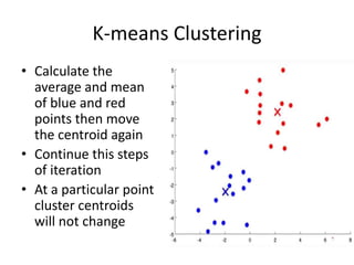
  K-means Clustering • Calculatethe average and mean of blue and red points then move the centroid again • Continue this steps of iteration • At a particular point cluster centroids will not change
• 80.
  K-Means • Initial setof clusters randomly chosen. • Iteratively, items are moved among sets of clusters until the desired set is reached. • High degree of similarity among elements in a cluster is obtained. • Given a cluster Ki={ti1,ti2,…,tim}, the cluster mean is mi = (1/m)(ti1 + … + tim)
• 81.
  Social Network Analysis (SNA)
• 82.
  Social network analysisis: • a set of relational methods for systematically understanding and identifying connections among actors Introduction
• 83.
  • Actors (nodes,points, vertices): - Individuals, Organizations, Events … • Relations (lines, arcs, edges, ties): between pairs of actors. - Undirected (symmetric) / Directed (asymmetric) - Binary / Valued Basic concepts Network Components
• 84.
  1) Egocentered Networks •Data on a respondent (ego) and the people they are connected to. Measures: Size Types of relations Basic concepts Types of network data: Def: An ego-centered network, or Egonet represents the one-hop neighbourhood of the node of interest Or Egonet consists of particular node and its immediate neighbours
• 85.
  2) Complete Networks •Connections among all members of a population. • Data on all actors within a particular (relevant) boundary. • Never exactly complete (due to missing data), but boundaries are set • Ex: Friendships among workers in a company. Measures: Graph properties Density Sub-groups Positions Background Types of network data:
• 86.
  The unit ofinterest in a network are the combined sets of actors and their relations. We represent actors with points and relations with lines. Example: Social Network data a b c e d
• 87.
  In general, arelation can be: Undirected / Directed Binary / Valued a b c e d Undirected, binary Directed, binary a b c e d a b c e d Undirected, Valued Directed, Valued a b c e d 1 3 4 21 Social Network data
• 88.
  From pictures tomatrices Undirected, binary Directed, binary a b c d e a b c d e 1 1 1 1 1 1 1 a b c d e a b c d e 1 1 1 1 1 1 1 1 1 1 Basic Data Structures Social Network data a b c e d a b c e d
• 89.
  d e c Indirect connectionsare what make networks systems. One actor can reach another if there is a path in the graph connecting them. a b c e d f b f a Connectivity Measuring Networks
• 90.
  Distance is measuredby the (weighted) number of relations separating a pair, Using the shortest path. Actor “a” is: 1 step from 4 2 steps from 5 3 steps from 4 4 steps from 3 5 steps from 1 Distance & number of paths Measuring Networks a
• 91.
  An information network: Email exchanges withinthe Reagan white house, early 1980s (source: Blanton, 1995) Measuring Networks
• 92.
  Centrality refers to(one dimension of) location, identifying where an actor resides in a network. Centrality Measuring Networks Centrality is fairly straight forward: we want to identify which nodes are in the ‘center’ of the network. In the sense that they have many and important connections. Three standard centrality measures capture a wide range of “importance” in a network: Degree Closeness Betweenness
• 93.
  The most intuitivenotion of centrality focuses on degree. Degree is the number of lines, and the actor with the most lines is the most important: Centrality Measuring Networks
• 94.
  Centrality Measuring Networks Relative measureof Degree Centrality: 1 ),( )(' 1     n ppa PC ki n i kD Degree Centrality: ),()( 1 ki n i kD ppaPC  
• 95.
  A second measureis closeness centrality. An actor is considered important if he/she is relatively close to all other actors. Closeness is based on the inverse of the distance of each actor to every other actor in the network. Closeness Centrality: Relative Closeness Centrality Centrality Measuring Networks 1 1 )],([)(    ki n i kC ppdPC ),( 1 1 ),( )(' 1 1 1 ki n i ki n i kC ppd n n ppd PC                   
• 96.
  Closeness Centrality Centrality Measuring Networks
• 97.
  Betweenness Centrality: Model basedon communication flow: A person who lies on communication paths can control communication flow, and is thus important. Betweenness centrality counts the number of shortest paths between i and k that actor j resides on. b a C d e f g h Centrality Measuring Networks
• 98.
  Centrality Measuring Networks Betweenness centralitycan be defined in terms of probability (1/gij), CB(pk) = iij(pk) = = gij = number of geodesics that bond actors pi and pj. gij(pk)= number of geodesics which bond pi and pj and content pk. iij(pk) = probability that actor pk is in a geodesic randomly chosen among the ones which join pi and pj. Betweenness centrality is the sum of these probabilities (Freeman, 1979). )(* g 1 ij kij pg ij kij g )(pg Normalizad: C’B(pk) = CB(pk) / [(n-1)(n-2)/2]
• 99.
  Betweenness Centrality: Centrality Measuring Networks
• 100.
  If we wantto measure the degree to which the graph as a whole is centralized, we look at the dispersion of centrality: Freeman’s general formula for centralization (which ranges from 0 to 1):   )]2)(1[( )()(1 *     nn pCpC C n i iDD D Centralization Measuring Networks