1

1

• 1.
  The z-Transform R.Suresh Babu Asst.Prof/ECE KCET 14-07-2011
• 2.
  Content  Introduction  z-Transform  Zeros and Poles  Region of Convergence  Important z-Transform Pairs  Inverse z-Transform  z-Transform Theorems and Properties  System Function
• 3.
  The z-Transform Introduction
• 4.
  Why z-Transform?  A generalization of Fourier transform  Why generalize it? – FT does not converge on all sequence – Notation good for analysis – Bring the power of complex variable theory deal with the discrete-time signals and systems
• 5.
  The z-Transform z-Transform
• 6.
  Definition  The z-transform of sequence x(n) is defined by ∞ X ( z) = ∑ x ( n) z n = −∞ −n Fourier Transform  Let z = e−jω. ∞ X (e ) = jω ∑ x ( n )e n =−∞ − jω n
• 7.
  z-Plane ∞ ∑ x ( n) z −n Im X ( z) = n = −∞ z = e−jω ω ∞ Re jω X (e ) = ∑ x ( n )e n =−∞ − jω n Fourier Transform is to evaluate z-transform on a unit circle.
• 8.
  z-Plane Im X(z) z = e−jω ω Re Im Re
• 9.
  Periodic Property ofFT X(ejω) X(z) −π π ω Im Re Can you say why Fourier Transform is a periodic function with period 2π?
• 10.
  The z-Transform Zeros and Poles
• 11.
  Definition  Give a sequence, the set of values of z for which the z-transform converges, i.e., |X(z)|<∞, is called the region of convergence. ∞ ∞ | X ( z ) |= ∑ x ( n) z − n = n = −∞ ∑ | x(n) || z |− n < ∞ n = −∞ ROC is centered on origin and consists of a set of rings.
• 12.
  Example: Region ofConvergence ∞ ∞ | X ( z ) |= ∑ x ( n) z − n = n = −∞ ∑ | x(n) || z |− n < ∞ n = −∞ Im ROC is an annual ring centered on the origin. r Re Rx − <| z |< Rx + jω ROC = {z = re | Rx − < r < Rx + }
• 13.
  Stable Systems  A stable system requires that its Fourier transform is uniformly convergent. Im  Fact: Fourier transform is to evaluate z-transform on a unit circle. 1  A stable system requires the Re ROC of z-transform to include the unit circle.
• 14.
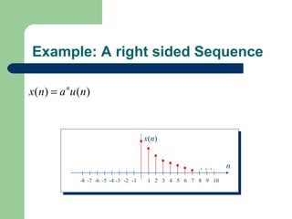
  Example: A rightsided Sequence x ( n) = a n u ( n) x(n) ... n -8 -7 -6 -5 -4 -3 -2 -1 1 2 3 4 5 6 7 8 9 10
• 15.
  Example: A rightsided Sequence For convergence of X(z), we x ( n) = a u ( n) n require that ∞ ∑ ∞ | az −1 | < ∞ | az −1 |< 1 X ( z) = ∑ a u (n)z n = −∞ n −n n =0 ∞ | z |>| a | = ∑ a n z −n ∞ 1 z n =0 X ( z ) = ∑ (az ) = −1 n −1 = ∞ n =0 1 − az z−a = ∑ (az −1 ) n | z |>| a | n =0
• 16.
  Example: A rightsided Sequence ROC for x(n)=anu(n) z X ( z) = z−a , | z |>| a | Which one is stable? Im Im 1 1 −a a −a a Re Re
• 17.
  Example: A leftsided Sequence x(n) = −a nu (−n − 1) -8 -7 -6 -5 -4 -3 -2 -1 1 2 3 4 5 6 7 8 9 10 ... n x(n)
• 18.
  Example: A leftsided Sequence For convergence of X(z), we x(n) = −a u (−n − 1)n require that ∞ ∞ X ( z ) = − ∑ a u (− n − 1)z ∑ | a −1 z | < ∞ −n | a −1 z |< 1 n n = −∞ −1 n =0 = − ∑ a n z −n n = −∞ | z |<| a | ∞ = −∑ a − n z n ∞ 1 z n =1 X ( z ) = 1 − ∑ (a z ) = 1 − −1 n −1 = ∞ n=0 1− a z z − a = 1 − ∑ a −n z n n =0 | z |<| a |
• 19.
  Example: A leftsided Sequence ROC for x(n)=−anu(− n−1) z X ( z) = z−a , | z |<| a | Which one is stable? Im Im 1 1 −a a −a a Re Re
• 20.
  The z-Transform Region of Convergence
• 21.
  Represent z-transform asa Rational Function P( z ) where P(z) and Q(z) are X ( z) = polynomials in z. Q( z ) Zeros: The values of z’s such that X(z) = 0 Poles: The values of z’s such that X(z) = ∞
• 22.
  Example: A rightsided Sequence z x ( n) = a n u ( n) X ( z) = , | z |>| a | z−a Im ROC is bounded by the pole and is the exterior a Re of a circle.
• 23.
  Example: A leftsided Sequence z x(n) = −a nu (−n − 1) X ( z) = , | z |<| a | z−a Im ROC is bounded by the pole and is the interior a Re of a circle.
• 24.
  Example: Sum ofTwo Right Sided Sequences x ( n) = ( 1 ) n u ( n) + ( − 1 ) n u ( n) 2 3 z z 2 z ( z − 12 ) 1 X ( z) = + = z−2 z+3 1 1 ( z − 1 )( z + 1 ) 2 3 Im ROC is bounded by poles and is the exterior of a circle. 1/12 −1/3 1/2 Re ROC does not include any pole.
• 25.
  Example: A TwoSided Sequence x(n) = (− 1 ) n u (n) − ( 1 ) n u (−n − 1) 3 2 z z 2 z ( z − 12 ) 1 X ( z) = + = z+3 z−2 1 1 ( z + 1 )( z − 1 ) 3 2 Im ROC is bounded by poles and is a ring. 1/12 −1/3 1/2 Re ROC does not include any pole.
• 26.
  Properties of ROC  A ring or disk in the z-plane centered at the origin.  The Fourier Transform of x(n) is converge absolutely iff the ROC includes the unit circle.  The ROC cannot include any poles  Finite Duration Sequences: The ROC is the entire z-plane except possibly z=0 or z=∞.  Right sided sequences: The ROC extends outward from the outermost finite pole in X(z) to z=∞.  Left sided sequences: The ROC extends inward from the innermost nonzero pole in X(z) to z=0.
• 27.
  More on Rationalz-Transform Consider the rational z-transform with the pole pattern: Im Find the possible a b c ROC’s Re
• 28.
  More on Rationalz-Transform Consider the rational z-transform with the pole pattern: Im Case 1: A right sided Sequence. a b c Re
• 29.
  More on Rationalz-Transform Consider the rational z-transform with the pole pattern: Im Case 2: A left sided Sequence. a b c Re
• 30.
  More on Rationalz-Transform Consider the rational z-transform with the pole pattern: Im Case 3: A two sided Sequence. a b c Re
• 31.
  More on Rationalz-Transform Consider the rational z-transform with the pole pattern: Im Case 4: Another two sided Sequence. a b c Re
• 32.
  The z-Transform Important z-Transform Pairs
• 33.
  Z-Transform Pairs Sequence z-Transform ROC δ(n) 1 All z All z except 0 (if m>0) δ( n − m ) z −m or ∞ (if m<0) 1 u (n) | z |> 1 1 − z −1 1 − u (−n − 1) | z |< 1 1 − z −1 1 n a u (n) | z |>| a | 1 − az −1 1 − a nu (−n − 1) | z |<| a | 1 − az −1
• 34.
  Z-Transform Pairs Sequence z-Transform ROC 1 − [cos ω0 ] z −1 [cos ω0 n]u (n) | z |> 1 1 − [ 2 cos ω0 ]z −1 + z −2 [sin ω0 ]z −1 [sin ω0 n]u (n) | z |> 1 1 − [2 cos ω0 ]z −1 + z −2 1 − [ r cos ω0 ]z −1 [r n cos ω0 n]u (n) | z |> r 1 − [ 2r cos ω0 ]z −1 + r 2 z − 2 [r sin ω0 ] z −1 [r n sin ω0 n]u (n) | z |> r 1 − [ 2r cos ω0 ]z −1 + r 2 z − 2 a n 0 ≤ n ≤ N −1 1− aN z−N  | z |> 0 0 otherwise 1 − az −1
• 35.
  The z-Transform Inverse z-Transform
• 36.
  The z-Transform z-Transform Theorems and Properties
• 37.
  Linearity Z [ x(n)] = X ( z ), z ∈ Rx Z [ y (n)] = Y ( z ), z ∈ Ry Z [ax(n) + by (n)] = aX ( z ) + bY ( z ), z ∈ Rx ∩ R y Overlay of the above two ROC’s
• 38.
  Shift Z [ x(n)] = X ( z ), z ∈ Rx Z [ x(n + n0 )] = z X ( z ) n0 z ∈ Rx
• 39.
  Multiplication by anExponential Sequence Z [ x(n)] = X ( z ), Rx- <| z |< Rx + −1 Z [a x(n)] = X (a z ) n z ∈| a | ⋅Rx
• 40.
  Differentiation of X(z) Z [ x(n)] = X ( z ), z ∈ Rx dX ( z ) Z [nx(n)] = − z z ∈ Rx dz
• 41.
  Conjugation Z[ x(n)] = X ( z ), z ∈ Rx Z [ x * (n)] = X * ( z*) z ∈ Rx
• 42.
  Reversal Z[ x(n)] = X ( z ), z ∈ Rx −1 Z [ x(−n)] = X ( z ) z ∈ 1 / Rx
• 43.
  Real and ImaginaryParts Z [ x(n)] = X ( z ), z ∈ Rx Re[ x(n)] = 1 [ X ( z ) + X * ( z*)] 2 z ∈ Rx Im [ x(n)] = 1 2j [ X ( z ) − X * ( z*)] z ∈ Rx
• 44.
  Initial Value Theorem x(n) = 0, for n < 0 x(0) = lim X ( z ) z →∞
• 45.
  Convolution of Sequences Z [ x(n)] = X ( z ), z ∈ Rx Z [ y (n)] = Y ( z ), z ∈ Ry Z [ x(n) * y (n)] = X ( z )Y ( z ) z ∈ Rx ∩ R y
• 46.
  Convolution of Sequences ∞ x ( n) * y ( n) = ∑ x(k ) y (n − k ) k = −∞  ∞ ∞  −n Z [ x(n) * y (n)] = ∑  ∑ x(k ) y (n − k )  z n = −∞  k = −∞  ∞ ∞ ∞ ∞ = ∑ x(k ) ∑ y(n − k )z −n = ∑ k = −∞ x(k ) z − k ∑ y (n)z − n n = −∞ k = −∞ n = −∞ = X ( z )Y ( z )
• 47.
  The z-Transform System Function
• 48.
  Shift-Invariant System x(n) y(n)=x(n)*h(n) h(n) X(z) H(z) Y(z)=X(z)H(z)
• 49.
  Shift-Invariant System X(z) Y(z) H(z) Y ( z) H ( z) = X ( z)
• 50.
  Nth-Order Difference Equation N M ∑a k =0 k y (n − k ) = ∑ br x(n − r ) r =0 N M Y ( z )∑ ak z − k = X ( z )∑ br z − r k =0 r =0 M N −r −k H ( z ) = ∑ br z ∑ ak z r =0 k =0
• 51.
  Representation in FactoredForm Contributes poles at 0 and zeros at cr M A∏ (1 − cr z −1 ) H ( z) = N r =1 ∏ (1 − d r z −1 ) k =1 Contributes zeros at 0 and poles at dr
• 52.
  Stable and CausalSystems Causal Systems : ROC extends outward from the outermost pole. Im M A∏ (1 − cr z −1 ) H ( z) = N r =1 Re ∏ (1 − d r z −1 ) k =1
• 53.
  Stable and CausalSystems Stable Systems : ROC includes the unit circle. Im M A∏ (1 − cr z −1 ) 1 H ( z) = N r =1 Re ∏ (1 − d r z −1 ) k =1
• 54.
  Example Consider the causalsystem characterized by y (n) = ay (n − 1) + x(n) Im 1 1 H ( z) = 1 − az −1 a Re h( n) = a n u ( n)
• 55.
  Determination of FrequencyResponse from pole-zero pattern  A LTI system is completely characterized by its pole-zero pattern. Im Example: p1 z − z1 e j ω0 H ( z) = ( z − p1 )( z − p2 ) z1 Re e jω0 − z1 p2 H (e jω0 ) = (e jω0 − p1 )(e jω0 − p2 )
• 56.
  Determination of FrequencyResponse from pole-zero pattern  A LTIjω |H(e )|=? pole-zero pattern. jω ∠H(e )=? system is completely characterized by its Im Example: p1 z − z1 e j ω0 H ( z) = ( z − p1 )( z − p2 ) z1 Re e jω0 − z1 p2 H (e jω0 ) = (e jω0 − p1 )(e jω0 − p2 )
• 57.
  Determination of FrequencyResponse from pole-zero pattern  A LTIjω |H(e )|=? pole-zero pattern. ∠H(e )=? system is completely characterized by its jω Im Example: p1 | | φ2 jω |H(e )| = e j ω0 | || | z1 φ1 φ3 Re ∠H(ejω) = φ1−(φ2+ φ3 ) p2
• 58.
  Example 1 20 H ( z) = −1 1 − az 10 dB 0 Im -1 0 0 2 4 6 8 2 1 a Re 0 -1 -2 0 2 4 6 8
• 59.
  Digital Signal Processing Applications DSP1-59
• 60.
  Image Processing Apollo
• 61.
  Magnetic Resonance Imaging(MRI)
• 62.
  Speech Processing “Speak& Spell” •Texas Instrument Speech/ Voice synthesizer •linear predictive coding (LPC) Memory Card DSP1-62
• 63.
  Towed array sensor SONAR(Sound navigation and ranging)
• 65.
  (Hearing aids)
• 67.
  Digital filter y [k] = h [ 0] x [k ] + h [1]x [k − 1] + h [2] x [k − 2] + h [3] x [k − 3] + h [ 4 ] x [k − 4 ] 4 = ∑ h [i ] x [k − i ] i =0
• 68.
  Echo Canceller
• 69.
  Acoustic Echo Canceller ผนังห้อง ระบบแฮนด์ฟรี โดยสำร Far-field ลำำโพง เครือข่ำย โทรศัพท์ ระบบ Near-field กำำจัด เอคโค่ ไมโครโฟน
• 70.
  Wireless Communication
• 71.
  Equaliser
• 72.
  Training bits forGSM